AMISTAD Lab – A Mathematical Theory of Abductive Logic

Introduction and Overview of the Project

Hello everyone! Our names are Hana Ahmed, Meg Kaye, and Nico Espinosa Dice, and we are working with Prof. George Montañez in the AMISTAD Lab (Artificial Machine Intelligence = Search Targets Awaiting Discovery) to formulate a mathematical theory of abductive reasoning. We hope to produce a machine learning model and graphical representation of creative problem-solving using abduction. 

Many people are aware of induction and deduction as forms of logical reasoning. However, abduction is arguably the closest resemblance of day-to-day human reasoning processes. Abduction, while still loosely defined, is rooted in the generation of plausible explanatory hypotheses that are consistent with observed facts. The concept of abductive logic is generally associated with the mathematician and philosopher Charles Sanders (C.S.) Peirce, and is regularly applied in real-life problem-solving tasks, such as medical diagnosis and criminology.

Abduction, Deduction, and Induction

These forms of logical reasoning have key but sometimes confusing differences! We can best illustrate these differences by a well-known example. For deduction, imagine that you have a bag of beans, and you know for a fact that all beans in that bag are white. If you take a handful of beans from that bag without looking at them, you can deduce the result that those beans must be white. For induction, imagine that you have a bag full of beans that you know nothing about, and you reach in and take some beans, and find that all of the beans in your hand are white. You can then induce a rule that states that all of the beans in that bag are white. For abduction, imagine that you have a bag of beans where every bean in that bag is white, and someone hands you a handful of white beans and asks where they came from. In this instance, you can abduce that the white beans in your hand must have come from that bag, where all the beans are white. The differences are a bit subtle, but luckily we have found a clear way to display them: using graphical models.

Graphical Models

Drawing from Bayesian probability and E.T. Jaynes’s formalized integrations of probability theory with logical reasoning, our group aims to model probabilistic abduction as a means of optimizing abductive hypothesis and explanation generation. We have chosen to use graphical models to visually represent components and steps of the abductive process, which includes observed/given facts and hypotheses weighted by Bayesian conditioning. With directed graphical models, specifically continuous Bayesian Networks, we measure causal relationships between information and assess the plausibility of abductive hypotheses by comparing their conditional probability measures and structural patterns. 

Creative and Non-Creative Abduction

To help frame our thinking, we asked the question: how can abduction be creative? Creativity is defined by Dean Simonton as an idea that is novel, useful, and surprising. From this definition of creativity, we categorized abduction into two types: creative and non-creative.

Non-creative abduction focuses on hypothesis selection. We use our graphical model to define non-creative abduction, as this allows us to develop a more rigorous definition.

In the following figure, we have observed three effects, and their known values are labeled by the colored circle.

Figure: Visual Representation of Graphical Model with Observed Effects

The goal of our model in this simplified scenario is to “explain” the observed effects. The model accomplishes this by selecting a hypothesis – a set of nodes and their respective assumed values – that is deemed the “cause.” The hypothesis is selected from the power set of all nodes in the graph. For example, rain = true is a possible hypothesis. (Rain is a node in the graph, and true is its assumed value for this particular hypothesis). However, because there is a high conditional probability of the road wet = true given rain = true, this hypothesis would contradict the observation that road wet = false. Consequently, the model moves on to another possible hypothesis, sprinklers = true. Given sprinklers = true, the resulting probabilities of grass wet = true and sidewalk wet = true are high, which is consistent with their observed values. Therefore, the model would select sprinklers = true as the hypothesis.

Contrasting non-creative abduction is, of course, creative abduction. By the definition of creativity, the idea – in the case of our model, the hypothesis – must be novel. Therefore, creative abduction involves hypothesis generation. We will again use our graphical model to illustrate creative abduction, as it allows us to be more rigorous in our definition.

Figure: Example of Creative Abduction Through Hypothesis Generation

In the simplified example above, tree burned = true is the observed effect that the model is attempting to explain. It is also known, based on other background information, that forest fire = false. Thus, the model cannot select forest fire = true as a hypothesis. Alternatively, the model can select lightning = true as a hypothesis, and then generate an edge from the node lightning to the node tree burned. Naturally, the question arises: in a more complicated example involving more nodes, why do we construct an edge from lightning to tree burned? How will we know that this edge is appropriate? In short, we use similarity.

Similarity Implementations

Adhering to our definition of creative abduction, we have developed methods of similarity scoring to measure the novelty of creative abductive hypotheses within our graphical model. Our two primary modes of similarity measurement, the Jaccard Index and graph edit distance, can be applied towards comparing the design and probabilistic weights of a graphical model’s structural components.

We have been testing the efficiency and accuracy of our similarity algorithms when applied to weighted Bayesian Networks and abductive reasoning models. From our experiment results, we will assess the overall similarity distribution dataset for trends and observations presented by either metric when applied to graphical models and various graphical structures. 

Comparing the Similarity of Edit Distance and Jaccard Index with Graph Paths

In this experiment, we decided to see how similarity dropped off as you traversed a path. We compared a source node to each node in increment steps along a path (with randomized weights), and graphed the results for both similarity metrics. For edit distance, since we are using a cost metric, a similarity of 0 is that they are the same node and a similarity of 1 is that they have no similarity. So, to compare edit distance and Jaccard index, we graphed 1 - edit distance.

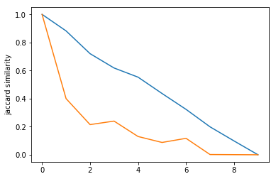
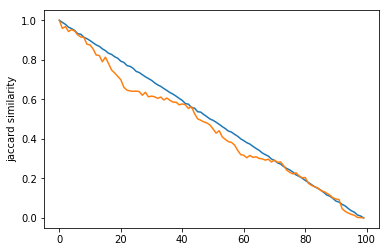
       Figure: 10 node paths     Figure: 100 node paths

Blue: 1 - edit distance

Orange: Jaccard index

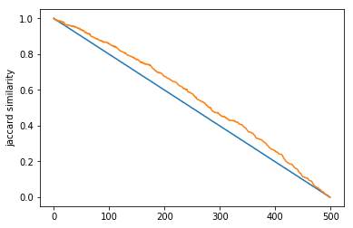
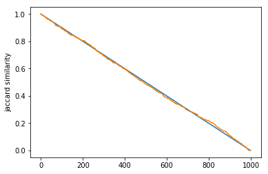
       Figure: 500 node paths     Figure: 1000 node paths

Blue: 1 - edit distance

Orange: Jaccard index

As you can see, both similarity metrics seemed to drop off at a linear rate as we traversed down the path, even at the smaller graphs. Although, the Jaccard index line definitely varied as the weights were changed and decided randomly for each run. However, the edit distance seemed to approach linearity much faster than the Jaccard index, which is an interesting find that highlights the difference between the two methods! Does this mean that edit distance is more reliable for smaller graphs, but less weighting-sensitive? It is definitely interesting to consider!

Similarity Distribution in Random Graphs

We are also analyzing the distribution of similarity in random graphs: how much does similarity vary in randomly generated graphs with the same number of nodes and edges?

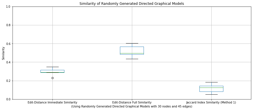
Figure: Similarity of Randomly Generated Directed Graphical Models

We are currently investigating how these distributions change with varying graph sizes. 

Similarity vs. Graph Size

Additionally, we are investigating how similarity varies with the size of graphs, measured by the number of nodes. 

Figure: Similarity vs. Graph Size

We are still investigating this question, and we are currently experimenting with a greater range of graph sizes.

Our Next Steps

We are planning on creating code to test some toy examples, and then progressively more complicated hypotheses. We also would like to do a bit more experimentation with the similarity metrics, specifically some of the ones that are built-in to Networkx (the Python package we are using to graph) to see how the different metrics fare under different conditions, with different types of graphs, etc. This has been a super fun research project so far, and we cannot wait to see where it takes us! 

Team

Lab Director: Prof. George Montañez

Hana Ahmed (hahmed7816@scrippscollege.edu)

Megan Kaye (mkaye@hmc.edu)

Nico Espinosa Dice (nespinosadice@hmc.edu)